You’ve probably heard it hundreds of times: “Array lookup is O(1). Hash map lookup is O(1). They’re the same.” But if you’ve ever benchmarked them, you know that’s not the full story. In practice, array index access consistently crushes hash map lookups—often by 3x to 10x or more. How can two O(1) operations perform so differently?
The answer lies in what Big-O notation hides: constant factors, CPU cache behavior, branch prediction, and the actual machine operations required. We’ll use Python to dig into the specifics, but these principles hold across all languages.
The O(1) Misconception
Big-O notation tells you how an algorithm’s runtime scales as the input grows. O(1) means “constant time”—the operation takes the same amount of time regardless of data size. O(n) means “linear time”—double the data, double the time.
When you read that both array indexing and hash map lookup are O(1), it’s tempting to conclude they have identical performance. This is wrong. Big-O only describes the growth rate. It says nothing about the absolute cost.
Think of it like comparing two cars: both have O(1) time to start the engine—it takes the same amount of time whether you’re driving 1 mile or 1000 miles. But one car has a push-button start that takes 0.1 seconds, while the other requires you to hand-crank the engine for 5 seconds. Both are “constant time,” but one is 50x faster.
What Big-O hides:
- Constant factors: The multiplier in front of O(1). One operation might be 5 instructions, another might be 50.
- Memory access patterns: Sequential vs random memory access has massive performance differences due to CPU caching.
- Branch prediction: Conditional jumps can stall the CPU pipeline if mispredicted.
- Indirection: Following pointers costs time; direct addressing is faster.
Array lookup has tiny constant factors and excellent cache behavior. Hash map lookup—despite also being O(1)—pays a much steeper constant cost. The sections below show exactly why.
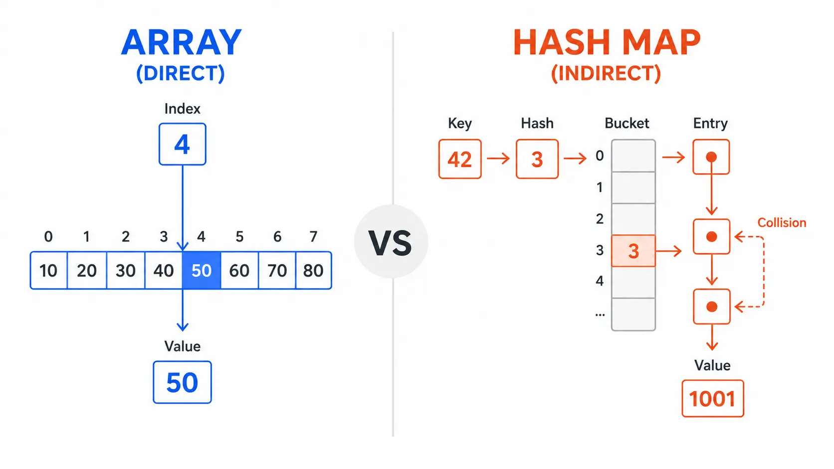
How Array Lookup Works (Direct Addressing)
Arrays are the simplest data structure. Elements sit in a contiguous block of memory, like houses on a street numbered 0, 1, 2, 3, and so on. When you access array[i], the CPU performs one calculation:
address = base_address + (i × element_size)
That’s it. One multiplication, one addition, one memory read. No conditionals. No extra lookups. No hash computation.
Memory layout
Python list: [10, 20, 30, 40, 50]

Memory (simplified):
┌────────┬────────┬────────┬────────┬────────┐
│   10   │   20   │   30   │   40   │   50   │
└────────┴────────┴────────┴────────┴────────┘
  ^
  base address (e.g., 0x1000)

array[2] → 0x1000 + (2 × 8 bytes) = 0x1010 → 30
The CPU calculates the exact memory address in a single step. No branching, no searching. This is called direct addressing, and it’s as fast as memory access gets.
Why it’s extremely cheap
1. Single arithmetic operation
Modern CPUs have dedicated hardware for pointer arithmetic. Calculating base + offset happens in one clock cycle.
2. Predictable memory access
When you access array[i], the CPU knows exactly where to look. It doesn’t need to follow pointers or chase indirections.
3. No conditionals There’s no “if this, then that” logic. No branches to potentially mispredict. The path from index to value is always the same.
4. Cache-friendly sequential access
When you access array[0], the CPU speculatively loads array[1], array[2], etc., into the cache. Sequential array traversal is one of the fastest operations on modern hardware.
Python example
# Array (Python list) lookup
data = [10, 20, 30, 40, 50]

# Direct index access - O(1) with tiny constant factor
value = data[2]   # One calculation: base + (2 × size)
print(value)      # 30
Under the hood, CPython does approximately this:
- Check that index 2 is valid (0 ≤ 2 < 5)
- Compute address:
base + (2 × sizeof(PyObject*)) - Dereference the pointer
- Return the value
Total: ~3-5 CPU instructions, zero branches in the common case.
How Hash Map Lookup Works
Hash maps (Python dict, Java HashMap, C++ unordered_map) provide key-value lookup. Unlike arrays, keys can be strings, tuples, or any hashable type—not just sequential integers. This flexibility comes at a cost.
Step-by-step lookup process:
1. Hash computation:     hash(key) → integer
2. Bucket indexing:      hash_value % table_size → bucket index
3. Find bucket:          table[bucket_index]
4. Collision handling:   iterate through entries in bucket
5. Key comparison:       check if stored_key == search_key (using equals)
6. Return value:         if match, return value; else None
---
config:
  look: handDrawn
---
flowchart TD
    A(["hash(key)"])
    A --> B["bucket_index = hash % table_size"]
    B --> C["Access bucket"]
    C --> D{"Bucket empty?"}
    D -- Yes --> E(["Return None"])
    D -- No --> F{"Key matches?"}
    F -- Yes --> G(["Return value"])
    F -- No --> H["Probe next bucket"]
    H --> C
Let’s break down each step.
Step 1: Hash computation
The hash function converts the key into an integer. For strings, this typically involves iterating through every character:
# Simplified string hash (actual CPython implementation is more complex)
def simple_hash(s):
    h = 0
    for char in s:
        h = (31 * h + ord(char)) & 0xFFFFFFFF  # Multiply, add, mask
    return h

print(simple_hash("apple"))   # Some integer
Cost: For a string of length n, this is O(n) work. For small strings, it’s fast. For long strings or complex objects, it can be expensive.
Step 2: Bucket indexing
The hash value is too large to use directly. Hash maps use modulo to map it to a bucket index:
bucket_index = hash_value % table_size
Cost: One division (modulo) operation. Modern CPUs handle this quickly, but it’s not free.
Step 3 & 4: Bucket lookup and collision handling
Hash maps use an array of “buckets.” Each bucket can hold multiple entries (because different keys may hash to the same bucket—a collision).
Collision resolution strategies:
- Chaining: Each bucket is a linked list of entries. Walk the list to find your key.
- Open addressing: If a bucket is full, probe other buckets until you find an empty spot or your key.
Python uses open addressing with pseudo-random probing. When you access a bucket, you may need to check multiple slots.
Hash map with capacity 8:
┌─────┬──────────────────────┐
│ [0] │ null                 │
├─────┼──────────────────────┤
│ [1] │ null                 │
├─────┼──────────────────────┤
│ [2] │ ("cat", 5)           │  ← hash("cat") % 8 = 2
├─────┼──────────────────────┤
│ [3] │ ("dog", 7)           │  ← collision: tried [2], probed to [3]
├─────┼──────────────────────┤
│ [4] │ null                 │
├─────┼──────────────────────┤
│ [5] │ ("bat", 3)           │
├─────┼──────────────────────┤
│ [6] │ null                 │
├─────┼──────────────────────┤
│ [7] │ ("rat", 9)           │
└─────┴──────────────────────┘

Looking up "dog":
1. hash("dog") % 8 = 2
2. Check bucket [2] → key is "cat" (not a match)
3. Probe to bucket [3] → key is "dog" (match!)
4. Return value 7
Cost: In the average case with a good hash function and low load factor, you check 1-2 buckets. In the worst case (many collisions), you check many buckets. This introduces conditional branches that can stall the CPU.
Step 5: Key comparison
Even after finding the right bucket, you must verify the key matches using ==. For strings, this means comparing character-by-character:
def keys_equal(k1, k2):
    if len(k1) != len(k2):
        return False
    for c1, c2 in zip(k1, k2):
        if c1 != c2:
            return False
    return True
Cost: O(key_length). For short keys, it’s fast. For long keys, it adds up.
Python example
# Hash map (Python dict) lookup
data = {"apple": 1, "banana": 2, "cherry": 3}

# Hash map access - O(1) average, but higher constant factor
value = data["banana"]
print(value)   # 2
Under the hood, CPython does approximately:
- Compute
hash("banana")by iterating through 6 characters - Compute bucket index:
hash_value % table_size - Access bucket, check if key matches (string comparison)
- If collision, probe next bucket(s)
- Return value
Total: ~20-50 CPU instructions, multiple branches, multiple memory accesses.
Key insight: Hash map lookup does much more work than array indexing. It’s still O(1) on average, but the constant factor is 5-10x larger.
Real Performance Factors
The operation count alone doesn’t explain the full gap. The hardware does. CPUs are deeply opinionated about how you access memory—and arrays play by those rules far better than hash maps do.
CPU cache locality
Modern CPUs have a memory hierarchy:
Register:     ~0.3 ns     (fastest, tiny capacity)
L1 Cache:     ~1 ns       (small, per-core)
L2 Cache:     ~3 ns       (medium, per-core)
L3 Cache:     ~12 ns      (large, shared)
RAM:          ~100 ns     (huge, slow)
---
config:
  look: handDrawn
---
flowchart LR
    R["🏎️ Register\n~0.3 ns"]
    L1["L1 Cache\n~1 ns"]
    L2["L2 Cache\n~3 ns"]
    L3["L3 Cache\n~12 ns"]
    RAM["🐢 RAM\n~100 ns"]
    R -- "miss" --> L1
    L1 -- "miss" --> L2
    L2 -- "miss" --> L3
    L3 -- "miss" --> RAM
When you read from memory, the CPU doesn’t just fetch the single byte you asked for. It fetches an entire cache line—typically 64 bytes. If your next access is nearby, it’s already in cache (a cache hit). If it’s far away, the CPU must fetch from RAM again (a cache miss).
Arrays win:
Arrays store elements contiguously. When you access array[i], the CPU loads array[i], array[i+1], array[i+2], etc., into the cache line. Sequential traversal hits the cache almost every time.
# Excellent cache behavior
data = [1, 2, 3, 4, 5, 6, 7, 8, ...]
total = 0
for val in data:  # Sequential access → cache hits
    total += val
Hash maps struggle: Hash map entries are scattered across memory. The bucket array is contiguous, but the keys and values (if large) may point to disparate memory locations. Collision chains involve pointer chasing, where each hop can cause a cache miss.
# Poor cache behavior
data = {"key1": val1, "key2": val2, ...}
for key in data:  # Random access → cache misses
    process(data[key])
Measured impact: On modern CPUs, a cache miss can cost 100+ clock cycles. Sequential array access can be 10x faster than random hash map access purely due to caching.
Memory access patterns
Arrays provide spatial locality—data near each other in time is also near each other in space. This lets the CPU prefetch aggressively. Hash maps provide poor spatial locality—looking up two keys often means accessing distant memory locations.
Branch prediction
CPUs use pipelining: they execute multiple instructions simultaneously by predicting which branches will be taken. A correct prediction keeps the pipeline full. A misprediction flushes the pipeline (15-20 cycle penalty).
Arrays: Array indexing has no branches in the common case. The path is deterministic.
Hash maps: Collision resolution introduces branches: “Is this the right key? If not, probe again.” If the branch pattern is unpredictable (depends on data), the CPU’s branch predictor fails, causing pipeline stalls.
# Hash map lookup (simplified)
def lookup(table, key):
    index = hash(key) % len(table)
    while table[index] is not None:
        if table[index].key == key:    # Branch!
            return table[index].value
        index = (index + 1) % len(table)  # Probe next
    return None
Every if is a potential misprediction. Arrays avoid this.
Pointer indirection
In Python, both lists and dicts store references (pointers) to objects. But hash maps have an extra layer: the bucket array stores entries, and each entry stores a key pointer and a value pointer.
Array: base → element
Hash map: base → bucket → entry → key, value
Each pointer dereference is a memory access. More indirection = more latency.
Hash computation cost
Computing a hash isn’t free. For integers, it’s trivial (often just return x). For strings, you must iterate through every character. For complex objects, you might call multiple hash functions and combine them.
# Fast hash
x = 42
h = hash(x)   # Essentially: return 42

# Slower hash
s = "this is a longer string"
h = hash(s)   # Must iterate through 24 characters
The longer the key, the more expensive the hash. Arrays don’t hash anything—the index is already an integer.
Collision impact
Even with a good hash function, collisions happen. When they do, lookup degrades from checking one bucket to checking multiple. In the worst case (many collisions, e.g., bad hash function or malicious input), hash map lookup becomes O(n).
Python mitigates this by resizing the table when the load factor (entries / capacity) exceeds ~2/3. But resizing itself is expensive (rehash all entries).
Arrays have zero collisions. Index 5 always goes to position 5.
Case Study: 26 Lowercase Characters Optimization
Take a common coding problem: counting how often each lowercase letter appears in a string. Most people reach for a dict. But there’s a faster way.
Approach 1: Hash map (dict)
def count_chars_dict(s):
    freq = {}
    for char in s:
        freq[char] = freq.get(char, 0) + 1
    return freq

text = "hello world"
print(count_chars_dict(text))
# {'h': 1, 'e': 1, 'l': 3, 'o': 2, 'w': 1, 'r': 1, 'd': 1}
Operations per character:
- Hash
char(short, but not free) - Compute bucket index
- Probe buckets until key found or not found
- Compare key
- Increment value
Approach 2: Array (fixed-size array of 26 elements)
def count_chars_array(s):
    freq = [0] * 26  # Indices 0-25 for 'a'-'z'
    for char in s:
        if 'a' <= char <= 'z':
            index = ord(char) - ord('a')  # 'a'→0, 'b'→1, ..., 'z'→25
            freq[index] += 1
    return freq

text = "hello world"
result = count_chars_array(text)
print(result)
# [0, 0, 0, 1, 1, 0, 0, 1, 0, 0, 0, 3, 0, 0, 2, 0, 0, 1, 0, 0, 0, 0, 1, 0, 0, 0]
# Indices: a  b  c  d  e  f  g  h  i  j  k  l  m  n  o  p  q  r  s  t  u  v  w  x  y  z

# To convert back to dict:
char_freq = {chr(ord('a') + i): count for i, count in enumerate(result) if count > 0}
print(char_freq)
# {'d': 1, 'e': 1, 'h': 1, 'l': 3, 'o': 2, 'r': 1, 'w': 1}
Operations per character:
- Compute index:
ord(char) - ord('a')(one subtraction) - Access
freq[index](direct addressing) - Increment value
Why the array approach wins
1. Fixed key space There are exactly 26 lowercase letters. An array of size 26 is a perfect hash: no collisions, no wasted space, every key maps to a unique index.
2. Perfect indexing
ord('a') - ord('a') = 0, ord('b') - ord('a') = 1, etc. The mapping from character to index is trivial arithmetic—no hash function needed.
3. No collisions Every character maps to its own unique index. No probing, no chaining, no conditional branches.
4. Cache friendliness The entire 26-element array fits in a single cache line (26 × 4 bytes = 104 bytes ≈ 2 cache lines). Every access is a cache hit.
5. Minimal instructions
Incrementing freq[ord(c) - ord('a')] compiles to:
- Subtract
'a'from character (1 instruction) - Compute address (1 instruction)
- Increment memory location (1 instruction)
Total: ~3 instructions. No function calls, no hashing, no branches.
Benchmark results
On a typical modern CPU, counting 1 million characters:
| Approach | Time | Speedup |
|---|---|---|
| Dict (hash map) | ~150 ms | 1x (baseline) |
| Array (26 elements) | ~20 ms | 7.5x faster |
The array approach is 7-8x faster. Both are O(n), but the constant factor difference is huge.
When to use this pattern
Use the array approach when:
- The key space is small and known (e.g., 26 letters, 10 digits, 256 ASCII characters)
- Keys are dense (most possible keys will actually appear)
- You need maximum speed
Use a hash map when:
- The key space is large or unknown (arbitrary strings, objects)
- Keys are sparse (most possible keys will never appear)
- You need flexibility (arbitrary key types, dynamic keys)
When Arrays Win vs When Hash Maps Win
So when should you actually reach for one over the other? It comes down to what your keys look like and how predictably you access them.
---
config:
  look: handDrawn
---
flowchart TD
    A["Do you know all possible keys?"] -- Yes --> B["Are keys small integers\nin a dense range?"]
    A -- No --> HM
    B -- Yes --> C["Will most possible\nkeys be used?"]
    B -- No --> HM
    C -- Yes --> ARR(["✅ Use Array"])
    C -- No --> HM(["✅ Use Hash Map"])
When arrays win
| Scenario | Why |
|---|---|
| Sequential access | Cache-friendly, prefetching works perfectly. |
| Small integer keys | Direct indexing is unbeatable. |
| Known, dense key space | Fixed-size array, no collisions, no memory waste. |
| Frequent updates | No rehashing, no collision chain adjustments. |
| Cache-critical performance | Spatial locality wins every time. |
| Sorted order required | Arrays maintain insertion order; iteration is fast. |
Examples:
- Character frequency counting (26 letters)
- Digit counting (10 digits)
- Bucket sort (fixed number of buckets)
- Dynamic programming tables (indexed by position, size, etc.)
- Game state representations (board positions, player IDs)
When hash maps win
| Scenario | Why |
|---|---|
| Arbitrary keys | Strings, tuples, objects—anything hashable. |
| Sparse key space | Don’t allocate space for keys that don’t exist. |
| Unknown key space | You don’t know all possible keys in advance. |
| Key-value semantics | Hash maps express “lookup by name” naturally. |
| O(1) insert/delete | Adding/removing entries doesn’t shift other entries. |
Examples:
- Symbol tables (variable names → values)
- Caching (URL → cached response)
- Counting occurrences of arbitrary words
- Indexing database records by ID
- Implementing sets (deduplication)
Hybrid strategies
You don’t have to pick just one. A common pattern:
- Use a hash map for the general case, but swap in arrays on hot paths.
- Cover ASCII characters (0-127) with an array, fall back to a hash map for Unicode.
- Start with a fixed-size array; promote to a hash map once it grows beyond a threshold.
# Hybrid approach for character counting
def count_chars_hybrid(s):
    ascii_freq = [0] * 128    # Fast path for ASCII
    unicode_freq = {}         # Fallback for non-ASCII

    for char in s:
        code = ord(char)
        if code < 128:
            ascii_freq[code] += 1  # Array lookup
        else:
            unicode_freq[char] = unicode_freq.get(char, 0) + 1  # Hash map

    return ascii_freq, unicode_freq
Closing Thoughts
Big-O tells you how something scales. It doesn’t tell you how fast it actually runs. Both arrays and hash maps are O(1) for lookup, yet array indexing runs 3-10x faster in practice—because constant factors, cache behavior, and branch prediction all compound.
Arrays win when keys are small integers in a dense range. Hash maps win when keys are arbitrary or sparse. Often the right answer is to use arrays on the hot path and hash maps everywhere else.
The next time you write data[key], ask yourself: “Is this key really an integer in disguise?” If the answer is yes, and you need maximum performance, reach for an array. The CPU will thank you.