Your API was humming along at 40ms response time for months. Black Friday hits. Same endpoint now takes 2 seconds. The operations team spins up more servers. Latency gets worse. Database CPU sits at 90%. Engineers blame the infrastructure team. Infrastructure blames the query. Everyone’s looking at dashboards instead of execution plans. Meanwhile, a single missing index on a 500M-row table is scanning the entire dataset on every request, and a WHERE LOWER(email) = ? clause is bypassing the index that actually exists.
Most SQL performance problems are not infrastructure problems. They are query planning problems, data access problems, and schema design problems. You cannot scale your way out of a sequential scan on a billion-row table. This article explains how PostgreSQL actually executes your SQL queries, how the query planner makes decisions, how to read execution plans to find bottlenecks, and how to systematically optimize slow queries in production systems.
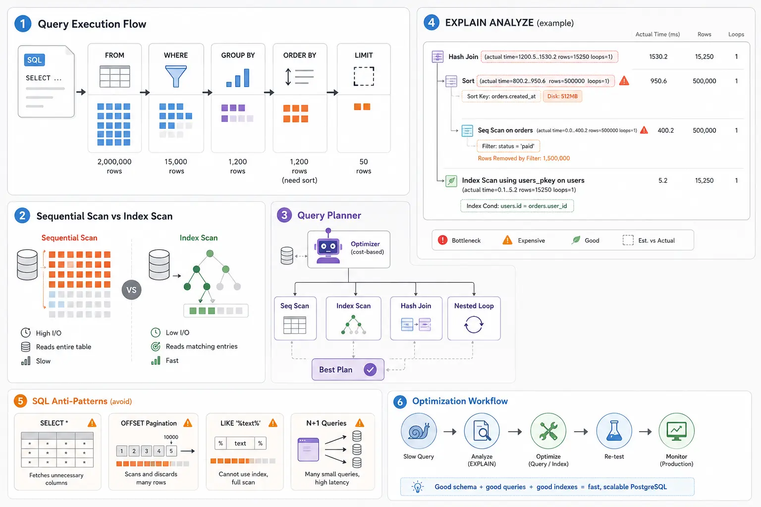
SQL Logical Execution Order — Why Syntax Lies
SQL is a declarative language. You write what you want, not how to get it. But PostgreSQL doesn’t execute your query in the order you wrote it. Understanding the logical execution order is the foundation for understanding why queries are slow.
The order you write SQL:
SELECT user_id, COUNT(*) as order_count
FROM orders
WHERE status = 'completed'
GROUP BY user_id
HAVING COUNT(*) > 5
ORDER BY order_count DESC
LIMIT 10;
The order PostgreSQL executes it:
- FROM — Identify the source table(s)
- JOIN — Combine tables if needed (Cartesian product, then filtered)
- WHERE — Filter rows before aggregation
- GROUP BY — Partition remaining rows into groups
- HAVING — Filter groups after aggregation
- SELECT — Compute expressions and projections
- DISTINCT — Remove duplicate rows (requires sort or hash)
- ORDER BY — Sort the result set
- LIMIT / OFFSET — Slice the sorted results
This execution order determines performance characteristics. WHERE filters before GROUP BY, so filtering early reduces aggregation cost. HAVING filters after aggregation, so it cannot leverage indexes the same way. ORDER BY happens late, meaning PostgreSQL might sort millions of rows even if you only want 10.
Why this matters for performance:
-- BAD: Filtering after aggregation
SELECT user_id, COUNT(*) as order_count
FROM orders
GROUP BY user_id
HAVING user_id IN (SELECT user_id FROM premium_users);

-- GOOD: Filtering before aggregation
SELECT o.user_id, COUNT(*) as order_count
FROM orders o
WHERE o.user_id IN (SELECT user_id FROM premium_users)
GROUP BY o.user_id;
The first query groups all orders (expensive), then filters. The second filters first (cheap), then groups only relevant rows. If you have 10M orders but only 1K premium users with 50K orders, the second query processes 50K rows instead of 10M.
Mental model for execution flow:
flowchart TD
    Start[SQL Query] --> From[1. FROM
Load base table]
    From --> Join[2. JOIN
Combine tables]
    Join --> Where[3. WHERE
Filter rows]
    Where --> Group[4. GROUP BY
Partition into groups]
    Group --> Having[5. HAVING
Filter groups]
    Having --> Select[6. SELECT
Compute expressions]
    Select --> Distinct[7. DISTINCT
Remove duplicates]
    Distinct --> Order[8. ORDER BY
Sort results]
    Order --> Limit[9. LIMIT/OFFSET
Slice results]
    Limit --> Result[Final Result]

    style Where fill:#90EE90
    style Group fill:#FFD700
    style Order fill:#FFB6C1
    style Limit fill:#87CEEB
Why ORDER BY + LIMIT is expensive:
-- This still sorts ALL orders, then takes 10
SELECT * FROM orders ORDER BY created_at DESC LIMIT 10;
Even with LIMIT 10, PostgreSQL must examine enough rows to determine which 10 are “first” after sorting. If there’s no index on created_at, it scans the entire table, sorts it, then returns 10 rows. An index on created_at DESC allows index-only retrieval of the first 10 without sorting.
Why LIMIT without ORDER BY is unpredictable:
-- Returns 10 random rows (physical storage order)
SELECT * FROM orders LIMIT 10;
Without ORDER BY, you get whatever rows PostgreSQL encounters first during the scan. This is typically insertion order but is not guaranteed. Physical row order changes after VACUUM, updates, or index scans.
PostgreSQL Query Planner Internals — How Execution Plans Are Built
The query planner is PostgreSQL’s optimizer. It takes your SQL, generates possible execution strategies, estimates cost for each, and picks the “cheapest” one. Understanding how it works explains why sometimes it makes bad decisions and how to fix them.
Planner vs Executor:
- Planner: Analyzes the query, estimates costs, generates execution plan (happens once per query)
- Executor: Follows the plan, retrieves data, computes results (happens for every execution)
Cost estimation model:
PostgreSQL estimates cost in arbitrary units (not milliseconds). The cost model considers:
- seq_page_cost (1.0) — Cost of sequential disk read
- random_page_cost (4.0) — Cost of random disk read
- cpu_tuple_cost (0.01) — Cost of processing one row
- cpu_operator_cost (0.0025) — Cost of applying one operator
These values are tunable but rarely changed. The ratio matters: random I/O is 4x more expensive than sequential I/O by default.
Cardinality estimation:
The planner estimates how many rows each operation will return. These estimates guide join strategy selection and index usage decisions. Bad estimates cause bad plans.
-- Planner estimates rows using table statistics
EXPLAIN SELECT * FROM orders WHERE status = 'completed';
-- Seq Scan on orders (cost=0.00..1847.00 rows=50000 width=120)
Statistics come from ANALYZE, which samples table data to estimate column distributions. If statistics are stale, estimates are wrong.
Common scan types and when to use them:
Sequential Scan
Reads the entire table from start to finish.
When chosen:
- No usable index exists
- Query touches >10-15% of table rows
- Table is small (<1000 rows)
Cost characteristics: O(n) where n is table size. Efficient for large result sets because of sequential I/O.
-- Forces sequential scan
SELECT * FROM orders WHERE EXTRACT(YEAR FROM created_at) = 2024;
-- Index on created_at exists but cannot be used (function blocks it)
Index Scan
Uses an index to find specific rows, then fetches them from the table.
When chosen:
- Query is selective (<5-10% of rows)
- Index exists on WHERE/JOIN columns
- Order matches index (for ORDER BY)
Cost characteristics: O(log n + m) where m is result set size. Each row requires a random I/O.
-- Index scan on orders_user_id_idx
SELECT * FROM orders WHERE user_id = 12345;
-- Returns 50 rows out of 10M (highly selective)
Bitmap Index Scan
Builds a bitmap of matching row locations, then fetches rows in physical order.
When chosen:
- Multiple indexes can be combined (OR/AND)
- Selectivity is moderate (5-25% of rows)
- Reduces random I/O by sorting fetches
Cost characteristics: Two-phase: build bitmap, then fetch rows sequentially.
-- Bitmap scan combines two indexes
SELECT * FROM orders
WHERE user_id = 12345 OR merchant_id = 67890;

-- Plan:
-- BitmapOr
--   -> Bitmap Index Scan on orders_user_id_idx
--   -> Bitmap Index Scan on orders_merchant_id_idx
-- -> Bitmap Heap Scan on orders
Index Only Scan
Retrieves all needed columns directly from the index without touching the table.
When chosen:
- All selected columns are in the index (covering index)
- Visibility map indicates pages are all-visible
- Index is smaller than table
Cost characteristics: O(log n + m) with no heap access. Fastest scan type.
-- Index only scan if index exists on (user_id, created_at)
SELECT user_id, created_at FROM orders WHERE user_id = 12345;
Join strategies:
Nested Loop Join
For each row in the outer table, scan the inner table.
When chosen:
- Small outer table, indexed inner table
- Highly selective joins
Cost characteristics: O(n × m) but with index lookup becomes O(n × log m).
-- Nested loop: 10 users × index lookup on orders
SELECT u.name, o.total FROM users u
JOIN orders o ON o.user_id = u.user_id
WHERE u.id IN (1,2,3,4,5);
Best for: Small outer input (< 1000 rows) with indexed inner table.
Hash Join
Builds a hash table from the smaller input, probes it for each row in the larger input.
When chosen:
- Equality joins on large tables
- No useful indexes
- Memory available for hash table
Cost characteristics: O(n + m) with memory overhead. Fast for large equi-joins.
-- Hash join: build hash table from smaller table
SELECT * FROM orders o
JOIN order_items oi ON oi.order_id = o.id
WHERE o.created_at > '2024-01-01';
Best for: Large tables with equality joins, sufficient work_mem.
Merge Join
Sorts both inputs, then merges them in sorted order.
When chosen:
- Inputs are already sorted (via index)
- Non-equality joins (>, <, BETWEEN)
- Memory constrained
Cost characteristics: O(n log n + m log m) if sorting needed, O(n + m) if pre-sorted.
-- Merge join on pre-sorted inputs
SELECT * FROM orders o
JOIN shipments s ON s.order_id >= o.id
WHERE o.status = 'completed';
Best for: Pre-sorted inputs or when hash join memory exceeds work_mem.
Join strategy comparison:
| Join Type | Best Use Case | Time Complexity | Memory Usage |
|---|---|---|---|
| Nested Loop | Small outer, indexed inner | O(n × log m) | Minimal |
| Hash Join | Large equi-joins | O(n + m) | High (hash table) |
| Merge Join | Pre-sorted inputs | O(n + m) | Medium (sort buffers) |
Why the planner sometimes chooses wrong:
- Stale statistics —
ANALYZEhasn’t run recently, cardinality estimates are wrong - Correlated columns — Planner assumes columns are independent (they’re not)
- Parameter sniffing — Prepared statements use generic plans that don’t adapt
- Cost model mismatch — Random page cost doesn’t reflect SSD performance
- Missing indexes — Planner can only choose from available access paths
Understanding EXPLAIN ANALYZE — Reading Execution Plans
EXPLAIN shows the planner’s chosen strategy. EXPLAIN ANALYZE actually executes the query and shows real metrics. This is your primary debugging tool for slow queries.
Basic EXPLAIN output:
EXPLAIN SELECT * FROM orders WHERE user_id = 12345;

-- Output:
Index Scan using orders_user_id_idx on orders
  (cost=0.42..125.34 rows=50 width=120)
  Index Cond: (user_id = 12345)
Key metrics explained:
- cost=0.42..125.34 — Startup cost..total cost (arbitrary units)
- Startup cost: work before returning first row
- Total cost: work to return all rows
- rows=50 — Estimated number of rows returned
- width=120 — Estimated average row size in bytes
- Index Cond — Condition used for index lookup
EXPLAIN ANALYZE adds actual metrics:
EXPLAIN ANALYZE SELECT * FROM orders WHERE user_id = 12345;

-- Output:
Index Scan using orders_user_id_idx on orders
  (cost=0.42..125.34 rows=50 width=120)
  (actual time=0.023..0.156 rows=48 loops=1)
  Index Cond: (user_id = 12345)
Planning Time: 0.123 ms
Execution Time: 0.198 ms
- actual time=0.023..0.156 — Real milliseconds (first row..last row)
- rows=48 — Actual rows returned (compare to estimated 50)
- loops=1 — How many times this node executed
- Planning Time — Time spent building the plan
- Execution Time — Time spent executing (not including network transfer)
EXPLAIN with buffers:
EXPLAIN (ANALYZE, BUFFERS)
SELECT * FROM orders WHERE user_id = 12345;

-- Additional output:
Buffers: shared hit=8 read=3
- shared hit=8 — Pages found in PostgreSQL’s shared buffer cache (RAM)
- read=3 — Pages read from disk
- written — Pages written (shows in INSERT/UPDATE)
Buffer metrics indicate I/O:
- All hits, no reads = data cached (fast)
- Many reads = cold cache or data doesn’t fit in memory (slow)
Identifying bottlenecks in complex queries:
EXPLAIN ANALYZE
SELECT u.name, COUNT(o.id) as order_count
FROM users u
LEFT JOIN orders o ON o.user_id = u.id
WHERE u.created_at > '2024-01-01'
GROUP BY u.id, u.name
ORDER BY order_count DESC
LIMIT 10;

-- Output (simplified):
Limit (cost=45123.45..45123.48 rows=10 width=48)
  (actual time=892.123..892.125 rows=10 loops=1)
  -> Sort (cost=45123.45..45873.45 rows=300000 width=48)
     (actual time=892.120..892.122 rows=10 loops=1)
     Sort Key: (count(o.id)) DESC
     Sort Method: top-N heapsort Memory: 25kB
     -> GroupAggregate (cost=0.42..38456.78 rows=300000 width=48)
        (actual time=0.125..765.234 rows=285000 loops=1)
        -> Nested Loop Left Join (cost=0.42..28456.78 rows=1000000 width=40)
           (actual time=0.023..512.456 rows=950000 loops=1)
           -> Index Scan using users_created_at_idx on users u
              (cost=0.42..5678.90 rows=300000 width=32)
              (actual time=0.015..45.123 rows=285000 loops=1)
              Index Cond: (created_at > '2024-01-01'::date)
           -> Index Scan using orders_user_id_idx on orders o
              (cost=0.42..3.12 rows=3 width=8)
              (actual time=0.001..0.001 rows=3 loops=285000)
              Index Cond: (user_id = u.id)
Planning Time: 1.234 ms
Execution Time: 892.345 ms
Reading this plan bottom-up:
- Users index scan — Fast (45ms), returns 285K users
- Orders index scan — Executes 285K times (loops=285000), 3 rows each time
- Nested Loop Join — Total 950K rows in 512ms (good)
- GroupAggregate — Groups 950K rows into 285K groups in 765ms
- Sort — Sorts 285K groups (slow part: 892ms total)
- Limit — Takes top 10
The bottleneck is the sort. PostgreSQL sorts 285K groups to find the top 10. This is unavoidable with GROUP BY + ORDER BY on aggregated values (no index can help).
Spotting bad cardinality estimates:
-- Bad estimate (estimated 50, actual 125000)
Index Scan using orders_status_idx on orders
  (cost=0.42..125.34 rows=50 width=120)
  (actual time=0.023..1523.456 rows=125000 loops=1)
  Index Cond: (status = 'completed')
Estimated 50 rows, got 125,000. The planner chose a nested loop join thinking the result set was small. It should have chosen a hash join. Fix: Run ANALYZE orders; to update statistics.
Detecting missing indexes:
-- Sequential scan on large table
Seq Scan on orders (cost=0.00..125678.00 rows=1 width=120)
  (actual time=145.234..3456.789 rows=1 loops=1)
  Filter: (email = 'user@example.com')
  Rows Removed by Filter: 4999999
Scanned 5M rows to find 1. The filter removed 4,999,999 rows. This screams for an index on email.
Detecting function calls blocking indexes:
-- Sequential scan despite index on email
Seq Scan on users (cost=0.00..5678.00 rows=1000 width=48)
  (actual time=0.023..156.234 rows=1 loops=1)
  Filter: (lower(email) = 'user@example.com')
Index exists on email but LOWER(email) is a function call. Create a functional index: CREATE INDEX ON users (LOWER(email));
Detecting disk spills:
-- Hash join spilling to disk
Hash Join (cost=5678.00..125678.00 rows=100000 width=48)
  (actual time=234.123..8956.789 rows=98453 loops=1)
  Hash Cond: (o.user_id = u.id)
  Buffers: shared hit=1234 read=5678 temp read=8765 written=8765
  -> Seq Scan on orders o
  -> Hash (cost=2345.00..2345.00 rows=50000 width=32)
     Buckets: 65536 Batches: 4 Memory Usage: 2048kB
temp read=8765 written=8765 means the hash table didn’t fit in work_mem and spilled to disk. This is slow. Fix: Increase work_mem for this query or optimize the join.
Practical EXPLAIN workflow:
- Run
EXPLAIN ANALYZEon slow query - Look at Execution Time — where did time go?
- Compare estimated rows vs actual rows — bad estimates?
- Check for Seq Scan on large tables — missing index?
- Look for high loops count — nested loop with wrong join?
- Check buffers — excessive disk reads?
- Look for temp read/written — memory spills?
Indexing Deep Dive — Making the Right Access Paths
Indexes are the primary tool for query optimization, but they’re not magic. Wrong indexes slow down writes and waste memory. Right indexes transform O(n) scans into O(log n) lookups.
B-tree indexes (default):
PostgreSQL’s default index type. Supports equality and range queries, handles NULL values, and maintains sorted order.
CREATE INDEX orders_user_id_idx ON orders (user_id);
-- Enables: WHERE user_id = ?
-- Enables: WHERE user_id IN (?, ?, ?)
-- Enables: ORDER BY user_id

CREATE INDEX orders_created_at_idx ON orders (created_at DESC);
-- Enables: WHERE created_at > ?
-- Enables: ORDER BY created_at DESC (no sort needed)
Composite (multi-column) indexes:
Order matters. Index on (a, b, c) can support:
WHERE a = ?WHERE a = ? AND b = ?WHERE a = ? AND b = ? AND c = ?
But NOT:
WHERE b = ?(first column not specified)WHERE a = ? AND c = ?(skips b)
-- Good composite index
CREATE INDEX orders_user_status_created_idx
ON orders (user_id, status, created_at DESC);

-- Query that uses all three columns
SELECT * FROM orders
WHERE user_id = 12345 AND status = 'completed'
ORDER BY created_at DESC;
Column ordering rules for composite indexes:
- Equality columns first —
WHERE x = ?columns before range columns - High cardinality before low — Selective columns before generic ones
- Range/sort columns last —
WHERE x > ?orORDER BY xat the end
-- BAD: range column first
CREATE INDEX bad_idx ON orders (created_at, user_id, status);

-- GOOD: equality columns first, range last
CREATE INDEX good_idx ON orders (user_id, status, created_at);
Covering indexes (index-only scans):
Include all columns needed by the query in the index to avoid table lookups.
-- Query needs user_id, status, and total
SELECT user_id, status, total FROM orders WHERE user_id = 12345;

-- Covering index includes total
CREATE INDEX orders_covering_idx
ON orders (user_id, status) INCLUDE (total);

-- Results in Index Only Scan (no heap access)
Partial indexes:
Index only rows that match a condition. Smaller, faster, and more efficient for specific queries.
-- Only index active orders
CREATE INDEX orders_active_idx ON orders (user_id, created_at)
WHERE status = 'active';

-- Query must match the WHERE clause
SELECT * FROM orders
WHERE user_id = 12345 AND status = 'active'
ORDER BY created_at DESC;
Partial indexes are excellent for:
- Soft-deleted records (
WHERE deleted_at IS NULL) - Active/pending states (
WHERE status IN ('active', 'pending')) - Recent records (
WHERE created_at > NOW() - INTERVAL '30 days')
GIN indexes (full-text search, arrays, JSONB):
Generalized Inverted Index. Handles multi-value columns.
-- Full-text search
CREATE INDEX articles_search_idx ON articles
USING GIN (to_tsvector('english', content));

-- Query
SELECT * FROM articles
WHERE to_tsvector('english', content) @@ to_tsquery('postgresql & performance');

-- Array containment
CREATE INDEX products_tags_idx ON products USING GIN (tags);
SELECT * FROM products WHERE tags @> ARRAY['electronics', 'sale'];

-- JSONB queries
CREATE INDEX users_metadata_idx ON users USING GIN (metadata);
SELECT * FROM users WHERE metadata @> '{"premium": true}';
BRIN indexes (block range indexes):
Extremely small indexes for large, naturally sorted tables (logs, time-series).
-- Logs table with 100M rows
CREATE INDEX logs_timestamp_brin_idx ON logs USING BRIN (timestamp);

-- Index size: ~100KB vs 2GB for B-tree
-- Query performance: Good for range scans on sorted data
SELECT * FROM logs WHERE timestamp > NOW() - INTERVAL '1 hour';
When to use BRIN:
- Table is large (>10M rows)
- Data is naturally sorted (insertion order matches query order)
- Queries are range-based, not point lookups
Trigram indexes (fuzzy text search):
For LIKE '%pattern%' queries with wildcards on both sides.
CREATE EXTENSION pg_trgm;

CREATE INDEX users_email_trgm_idx ON users
USING GIN (email gin_trgm_ops);

-- Now this query uses the index
SELECT * FROM users WHERE email LIKE '%@example.com';
Index maintenance costs:
Every index slows down writes. Each INSERT/UPDATE/DELETE must update all relevant indexes.
-- Table with 10 indexes
INSERT INTO orders (user_id, status, total, created_at, ...)
VALUES (12345, 'active', 99.99, NOW(), ...);

-- PostgreSQL must:
-- 1. Insert row into table
-- 2. Update orders_user_id_idx
-- 3. Update orders_status_idx
-- 4. Update orders_created_at_idx
-- ... (7 more indexes)
Index bloat:
Indexes grow over time due to updates and deletes. VACUUM doesn’t shrink indexes. Use REINDEX to rebuild bloated indexes.
-- Check index bloat
SELECT schemaname, tablename, indexname,
  pg_size_pretty(pg_relation_size(indexrelid)) as index_size
FROM pg_stat_user_indexes
ORDER BY pg_relation_size(indexrelid) DESC;

-- Rebuild bloated index
REINDEX INDEX CONCURRENTLY orders_user_id_idx;
Practical indexing strategy:
- Start with no indexes (except primary key and foreign keys)
- Identify slow queries from logs or monitoring
- Analyze execution plans to find sequential scans
- Create targeted indexes for those queries
- Measure impact — did query speed improve? Did write performance degrade?
- Remove unused indexes — check
pg_stat_user_indexes.idx_scan = 0
Common SQL Performance Anti-Patterns
These patterns destroy performance at scale. Each is common in production codebases, often introduced by developers who don’t understand query execution.
SELECT * — The Silent Performance Killer
-- BAD: Fetches all 50 columns
SELECT * FROM orders WHERE user_id = 12345;

-- GOOD: Fetches only needed columns
SELECT id, total, status, created_at FROM orders WHERE user_id = 12345;
Why this matters:
- Network transfer: 50 columns × 1000 rows = 50KB vs 4 columns = 4KB
- Memory usage: Application must allocate memory for all columns
- Index-only scans impossible: Index can’t cover
* - Breaks when schema changes: Adding a
BLOBcolumn kills allSELECT *queries
OFFSET Pagination — The N×Page Problem
-- BAD: Scans and discards 100,000 rows
SELECT * FROM orders ORDER BY created_at DESC LIMIT 20 OFFSET 100000;
OFFSET forces PostgreSQL to scan and discard all skipped rows. Page 5000 (offset 100,000) scans 100,020 rows to return 20.
Better: Keyset pagination (seek method)
-- First page
SELECT * FROM orders ORDER BY created_at DESC LIMIT 20;
-- Returns last created_at: '2024-03-15 10:30:00'

-- Next page (use last value as cursor)
SELECT * FROM orders
WHERE created_at < '2024-03-15 10:30:00'
ORDER BY created_at DESC LIMIT 20;
Keyset pagination scans only 20 rows per page regardless of page number. Works with any indexed column.
Functions on Indexed Columns — Index Bypass
-- BAD: Index on created_at cannot be used
SELECT * FROM orders WHERE DATE(created_at) = '2024-03-15';

-- GOOD: Use range query
SELECT * FROM orders
WHERE created_at >= '2024-03-15' AND created_at < '2024-03-16';
Any function call on a column prevents index usage. Alternative: create a functional index.
-- Functional index
CREATE INDEX orders_created_date_idx ON orders (DATE(created_at));

-- Now this works
SELECT * FROM orders WHERE DATE(created_at) = '2024-03-15';
But the range query is still better—it’s simpler and doesn’t require a special index.
Leading Wildcard LIKE — Untethered Search
-- BAD: Cannot use B-tree index
SELECT * FROM users WHERE email LIKE '%@example.com';

-- REQUIRES: Trigram index
CREATE INDEX users_email_trgm_idx ON users USING GIN (email gin_trgm_ops);
B-tree indexes work for prefix searches (LIKE 'abc%') but not suffix searches (LIKE '%abc'). Trigram indexes handle both but are larger and slower.
Better: Redesign the schema
-- Add a reversed email column or extract domain
ALTER TABLE users ADD COLUMN email_domain TEXT;
UPDATE users SET email_domain = split_part(email, '@', 2);
CREATE INDEX users_email_domain_idx ON users (email_domain);

-- Query
SELECT * FROM users WHERE email_domain = 'example.com';
OR Conditions — Planner Confusion
-- BAD: Planner struggles with OR
SELECT * FROM orders WHERE user_id = 12345 OR merchant_id = 67890;
The planner might choose a sequential scan instead of combining indexes. Better: Use UNION ALL to force index usage.
-- GOOD: Explicitly use both indexes
SELECT * FROM orders WHERE user_id = 12345
UNION ALL
SELECT * FROM orders WHERE merchant_id = 67890 AND user_id != 12345;
The user_id != 12345 prevents duplicates without requiring UNION (which deduplicates expensively).
Unnecessary DISTINCT — Hidden Sorting
-- BAD: DISTINCT requires sort or hash
SELECT DISTINCT user_id FROM orders WHERE status = 'completed';
If user_id already has no duplicates in the result (due to GROUP BY or unique index), DISTINCT is wasteful overhead.
When DISTINCT is needed:
- Joining tables that create duplicates
- Aggregating non-unique columns
When DISTINCT is wasteful:
- Result already unique due to primary key or unique constraint
- Can use
GROUP BYinstead
N+1 Queries from ORMs — The Silent Killer
# BAD: 1 query for users + N queries for orders (N+1 problem)
users = db.query("SELECT * FROM users WHERE active = true")
for user in users:
    orders = db.query("SELECT * FROM orders WHERE user_id = ?", user.id)
    print(f"{user.name}: {len(orders)} orders")
This executes 1 + N queries. If there are 1000 users, that’s 1001 database round trips.
# GOOD: 2 queries total (or 1 with JOIN)
users = db.query("SELECT * FROM users WHERE active = true")
user_ids = [u.id for u in users]
orders = db.query("SELECT user_id, COUNT(*) FROM orders WHERE user_id IN (?) GROUP BY user_id", user_ids)
orders_map = {o.user_id: o.count for o in orders}

for user in users:
    print(f"{user.name}: {orders_map.get(user.id, 0)} orders")
Better: Use ORM eager loading (select_related, prefetch_related in Django, joinedload in SQLAlchemy).
Large JOIN Explosions — Cartesian Product Hell
-- BAD: Cartesian product between orders and order_items
SELECT * FROM orders o, order_items oi
WHERE o.status = 'completed' AND oi.product_id = 123;
Missing the join condition creates a Cartesian product. If orders has 1M rows and order_items has 5M rows, this produces 5 trillion rows before filtering.
-- GOOD: Explicit join condition
SELECT * FROM orders o
JOIN order_items oi ON oi.order_id = o.id
WHERE o.status = 'completed' AND oi.product_id = 123;
Always use explicit JOIN syntax. Avoid comma-separated tables in FROM.
Real Production Optimization Workflow
Optimizing SQL is not guessing and adding indexes. It’s a systematic debugging process.
Step 1: Detect the slow query
Use pg_stat_statements to find slow queries:
-- Enable pg_stat_statements
CREATE EXTENSION pg_stat_statements;

-- Find slowest queries by total time
SELECT
  query,
  calls,
  mean_exec_time,
  total_exec_time,
  rows
FROM pg_stat_statements
ORDER BY total_exec_time DESC
LIMIT 10;
Step 2: Run EXPLAIN ANALYZE
EXPLAIN (ANALYZE, BUFFERS)
<your slow query>;
Look for:
- Sequential scans on large tables
- High actual time vs estimated time
- Estimated rows vs actual rows mismatch
- Many buffer reads (disk I/O)
Step 3: Inspect scan types and row estimates
- Seq Scan on table with millions of rows → Need index
- Estimated 100 rows, actual 100,000 → Run
ANALYZE - Nested loop with 10,000 iterations → Wrong join strategy
Step 4: Check for stale statistics
-- Check when statistics were last updated
SELECT
  schemaname,
  tablename,
  last_analyze,
  last_autoanalyze
FROM pg_stat_user_tables
WHERE tablename = 'orders';

-- Manually update statistics
ANALYZE orders;
Step 5: Add or adjust indexes
Create targeted indexes based on WHERE/JOIN/ORDER BY clauses.
-- Query: WHERE user_id = ? AND status = ? ORDER BY created_at DESC
CREATE INDEX orders_user_status_created_idx
ON orders (user_id, status, created_at DESC);
Step 6: Reduce scanned rows
Sometimes you cannot make a query faster with indexes. Reduce the dataset instead.
- Add WHERE clauses to filter earlier
- Use partial indexes for common filters
- Partition large tables by time (e.g., monthly partitions)
- Archive old data to separate tables
Step 7: Re-test with EXPLAIN ANALYZE
EXPLAIN (ANALYZE, BUFFERS)
<your slow query>;
Compare before and after:
- Did execution time decrease?
- Did index get used?
- Did row estimates improve?
Step 8: Monitor for regressions
Queries that are fast today can become slow tomorrow due to:
- Data growth (table doubles in size)
- Data distribution changes (status=’active’ was 10%, now 50%)
- Statistics becoming stale
- Index bloat
Set up alerts for:
- Query execution time exceeds threshold
- Sequential scans on large tables
- Index scan row estimates off by >10×
Advanced PostgreSQL Optimization Topics
Partitioning
Split large tables into smaller chunks to improve query performance and maintenance.
-- Partition orders by month
CREATE TABLE orders (
  id BIGSERIAL,
  user_id INTEGER,
  total DECIMAL,
  created_at TIMESTAMP
) PARTITION BY RANGE (created_at);

-- Create monthly partitions
CREATE TABLE orders_2024_01 PARTITION OF orders
  FOR VALUES FROM ('2024-01-01') TO ('2024-02-01');

CREATE TABLE orders_2024_02 PARTITION OF orders
  FOR VALUES FROM ('2024-02-01') TO ('2024-03-01');

-- Queries automatically use relevant partition
SELECT * FROM orders WHERE created_at >= '2024-01-15';
-- Only scans orders_2024_01 partition
When to partition:
- Table exceeds 100GB
- Queries filter on a time-based column
- Need to drop old data efficiently (drop partition instead of DELETE)
Materialized Views
Pre-compute expensive queries and refresh periodically.
-- Expensive aggregation query
CREATE MATERIALIZED VIEW daily_revenue AS
SELECT
  DATE(created_at) as date,
  SUM(total) as revenue,
  COUNT(*) as order_count
FROM orders
WHERE status = 'completed'
GROUP BY DATE(created_at);

-- Create index on materialized view
CREATE INDEX daily_revenue_date_idx ON daily_revenue (date);

-- Refresh periodically (via cron or trigger)
REFRESH MATERIALIZED VIEW CONCURRENTLY daily_revenue;
When to use:
- Query is expensive (>1s execution time)
- Data doesn’t need to be real-time (staleness acceptable)
- Query is read frequently (>100/sec)
Connection Pooling
PostgreSQL uses process-per-connection. Too many connections exhaust resources.
Problem:
max_connections = 100
Each connection uses ~10MB RAM
100 connections = 1GB RAM just for connections
Solution: PgBouncer
PgBouncer maintains a pool of database connections and multiplexes client connections.
# pgbouncer.ini
[databases]
mydb = host=localhost port=5432 dbname=mydb

[pgbouncer]
pool_mode = transaction
max_client_conn = 1000
default_pool_size = 20
- Application opens 1000 connections to PgBouncer
- PgBouncer maintains 20 connections to PostgreSQL
- 50× reduction in database connections
Prepared Statements
Reuse query plans across executions to reduce planning overhead.
-- Normal query (planned every time)
SELECT * FROM orders WHERE user_id = 12345;
SELECT * FROM orders WHERE user_id = 67890;

-- Prepared statement (planned once)
PREPARE get_user_orders (INTEGER) AS
  SELECT * FROM orders WHERE user_id = $1;

EXECUTE get_user_orders(12345);
EXECUTE get_user_orders(67890);
Trade-off: Generic plans might be suboptimal for specific parameter values. PostgreSQL uses adaptive planning after 5 executions.
Query Caching
Cache query results in application layer (Redis, Memcached) to avoid database entirely.
def get_user_orders(user_id):
    cache_key = f"user_orders:{user_id}"
    result = redis.get(cache_key)

    if result is None:
        result = db.query("SELECT * FROM orders WHERE user_id = ?", user_id)
        redis.setex(cache_key, 300, result)  # Cache for 5 minutes

    return result
When to cache:
- Query results change infrequently
- Query is expensive
- Staleness is acceptable
Autovacuum Tuning
VACUUM reclaims space from deleted rows and updates statistics. Autovacuum does this automatically but may need tuning.
-- Check autovacuum settings
SHOW autovacuum_vacuum_scale_factor;  -- Default: 0.2 (20%)
SHOW autovacuum_analyze_scale_factor; -- Default: 0.1 (10%)

-- Tune for high-churn table
ALTER TABLE orders SET (
  autovacuum_vacuum_scale_factor = 0.05,  -- Vacuum at 5% updates
  autovacuum_analyze_scale_factor = 0.02  -- Analyze at 2% updates
);
VACUUM vs VACUUM FULL:
VACUUM— Marks space as reusable, fast, no locksVACUUM FULL— Rewrites entire table, slow, exclusive lock
Use VACUUM FULL only during maintenance windows for severely bloated tables.
HOT Updates and Fillfactor
Heap-Only Tuple (HOT) updates optimize in-place updates when indexed columns don’t change.
-- Set fillfactor to leave space for updates
ALTER TABLE orders SET (fillfactor = 80);

-- Now updates that don't change indexed columns are faster
UPDATE orders SET status = 'shipped' WHERE id = 123;
Fillfactor = 80 leaves 20% free space per page for updates, reducing page splits and fragmentation.
Parallel Query Execution
PostgreSQL can parallelize large scans and aggregations.
-- Enable parallel query
SET max_parallel_workers_per_gather = 4;

-- Large sequential scan uses multiple workers
EXPLAIN SELECT COUNT(*) FROM orders;
-- Finalize Aggregate (actual time=123.45)
--   -> Gather (workers=4)
--        -> Partial Aggregate
--             -> Parallel Seq Scan on orders
Parallel execution helps with:
- Large sequential scans
- Large aggregations (SUM, COUNT, AVG)
- Large sorts
Production Engineering Lessons
These are insights from running PostgreSQL at scale in production systems.
The fastest query is the query never executed. Before optimizing a slow query, ask if it needs to run at all. Can you precompute results? Can you cache them? Can you denormalize to avoid joins? Optimization is not always about making queries faster—sometimes it’s about running fewer of them.
Reduce data movement. Every query moves data from disk → memory → CPU → network → application. The less data that moves, the faster the system. Filter early with WHERE. Select only needed columns. Use covering indexes to avoid heap access. Aggregate in the database instead of application.
Indexes are not free. Every index costs disk space and slows writes. Resist the temptation to index every column. Index strategically based on slow query analysis. Drop unused indexes—they cost you without helping.
ORMs hide complexity. Object-relational mappers generate SQL that is often inefficient. Always inspect generated queries using query logging or middleware. Lazy loading causes N+1 queries. Eager loading pulls unnecessary data. Write raw SQL for performance-critical paths.
Most scaling problems are data access problems. “We need more servers” is rarely the right answer. The right answer is usually “we need better indexes” or “we need to query less data.” Scaling out (horizontal scaling) is expensive and complex. Scaling up (better queries) is cheap and effective until you reach hardware limits.
Schema design affects performance for years. Poor schema choices compound over time. Nullable columns prevent optimizations. JSON fields hide relational structure. Wide tables with 100+ columns slow every query. Design schema with query patterns in mind from day one. Refactoring schema in a 500GB database is painful.
Premature optimization is dangerous, but late optimization is expensive. Don’t add indexes before you have slow queries. But don’t wait until the database is on fire. Monitor query performance continuously. Set up alerts for degradation. Fix slow queries when they first appear at 200ms, not when they reach 10s.
Data distribution matters as much as volume. A 10M row table with uniform distribution behaves differently from a 10M row table where 90% of rows have status=’archived’. Skewed data breaks planner assumptions. Use partial indexes, partitioning, or separate tables for hot/cold data.
Index maintenance is not optional. Indexes bloat over time from updates and deletes. Bloated indexes are larger and slower. Monitor index size growth. Run REINDEX CONCURRENTLY during maintenance windows. Vacuum regularly to keep statistics fresh.
Connection limits are real. PostgreSQL is process-per-connection. Every connection consumes memory and file descriptors. Opening 5000 connections to a database configured for 100 is a fast path to crashes. Use connection pooling (PgBouncer, PgPool). Set application-level connection limits. Monitor connection usage.
Closing Thoughts
SQL performance optimization is not magic. It is systematic analysis of how queries execute, understanding what the planner sees, and providing the tools it needs to make better decisions. Most performance problems come from sequential scans on large tables, missing indexes, stale statistics, or queries that move more data than necessary. The solution is rarely “buy faster hardware.” It is almost always “understand what the database is doing and give it a better path.”
The discipline of reading execution plans is the most valuable skill for database optimization. EXPLAIN ANALYZE shows you reality, not assumptions. It reveals where time is spent, where estimates are wrong, and where indexes would help. Every production engineer should be comfortable reading execution plans and understanding what they mean. This is not optional knowledge—it is the foundation of building systems that stay fast as data grows.
Start with the slow query log. Find the queries taking seconds. Read their execution plans. Look for sequential scans, bad cardinality estimates, and unnecessary sorts. Add targeted indexes. Re-measure. Repeat. This process, done consistently, keeps systems fast over time. There are no shortcuts, but the process works.
Questions
-
Why does PostgreSQL sometimes choose a sequential scan even when an index exists, and when is this actually the right choice?
-
How does the logical SQL execution order (WHERE before GROUP BY) influence which optimizations are possible and which indexes can be used?