Every programmer, at some point, needs to store a collection of items. A list of student scores. A sequence of daily temperatures. The names of passengers on a flight. Arrays are the most fundamental tool for the job — the first data structure most people learn and the one that underpins countless others. Yet it is easy to rush through arrays because they “feel simple,” and miss the depth they carry.
This guide builds arrays from first principles. You will understand what an array is and why it was designed the way it was, see real-world analogies that make the abstract concrete, walk through every common operation with honest time-complexity explanations, and learn the core techniques — two pointers, sliding window, prefix sum, and more — that turn arrays into a powerful problem-solving tool. Whether you are brand new to programming or brushing up before an interview, there is something here for you.
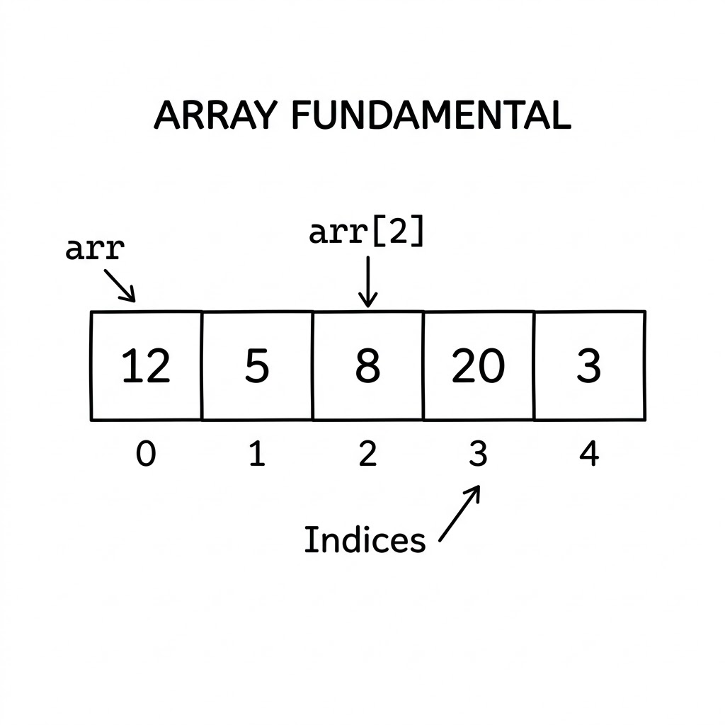
What is an Array?
Picture a row of identical mailboxes on a street. Each mailbox sits in a fixed position, has a number painted on it, and can hold exactly one item. You can walk straight to mailbox 7 without checking any of the others. That is an array.
Formally, an array is a contiguous block of memory that stores elements of the same type, each accessible by a numbered position called an index. “Contiguous” is the key word: all elements sit side by side in memory, with no gaps. This is what makes arrays fast.
Index-based access
Arrays use zero-based indexing in most languages, meaning the first element lives at index 0, the second at index 1, and so on. To read any element, you give the array its index, and the computer calculates the exact memory address in a single arithmetic step:
address = base_address + (index × element_size)
There is no scanning, no searching — just a multiplication and an addition. This is why reading from an array by index is O(1): it takes the same amount of time whether the array has 5 elements or 5 million.
---
config:
  look: handDrawn
---
flowchart LR
    subgraph Array["Array in memory"]
        direction LR
        I0["[0] - 42"] --- I1["[1] - 17"] --- I2["[2] - 85"] --- I3["[3] - 6"] --- I4["[4] - 31"]
    end
    P["base address (e.g. 0x1000)"] --> I0
In Python, arrays are represented by the built-in list type. Creating one is straightforward:
# Creating a list (Python's array equivalent)
scores = [42, 17, 85, 6, 31]

# Access by index
print(scores[0])   # 42 — first element
print(scores[4])   # 31 — last element
print(scores[-1])  # 31 — negative indexing also works in Python
Strengths and limits
Arrays have a clear set of trade-offs that you should understand before choosing them.
Strengths:
- O(1) random access — jump to any element instantly by index.
- Cache-friendly — elements sit next to each other in memory, so the CPU can prefetch them efficiently. Iterating through an array is one of the fastest operations on modern hardware.
- Simple and predictable — easy to reason about, easy to debug.
- Low memory overhead — just the elements themselves, no extra pointers or metadata per element.
Limits:
- Fixed size in static arrays — once allocated, a static array cannot grow. Dynamic arrays (like Python lists) work around this, but at a cost.
- Expensive insertion and deletion in the middle — adding or removing an element in the middle requires shifting all elements after it, which is O(n).
- Requires contiguous memory — if memory is fragmented, allocating a large array may fail even if there is enough total free space.
Real-life Analogies
Good analogies make abstract ideas concrete. Here are a few that map closely to how arrays actually work.
Theater seats
Imagine a single row of numbered seats in a theater: 1, 2, 3, …, 50. Each seat has exactly one position. The usher can take you directly to seat 27 without looking at any other seat. If you want to squeeze a new seat between 13 and 14, every seat from 14 onward must shift one position to the right — a disruptive, time-consuming shuffle.
This is precisely what arrays do. Fast access by position, expensive insertion in the middle.
Books on a shelf
A bookshelf where books are arranged in order by catalog number. Grabbing book number 5 is instant — you just count from the left. But if the library wants to insert a new book between positions 3 and 4, every book from position 4 onward must slide one spot to make room.
Parking slots in a lot
A single-row parking lot numbered from 1 to 100. The attendant can instantly see if slot 42 is free and assign it. But if the lot decides to add a new slot between 10 and 11, every car from slot 11 onward must move — impractical in a real lot, expensive in software.
Mapping to array concepts
| Real-life concept | Array concept |
|---|---|
| Seat number / slot number | Index |
| The item at a seat | Element |
| Jumping straight to seat 27 | O(1) random access |
| Shuffling seats to insert one | O(n) insertion |
| Removing a seat and sliding others | O(n) deletion |
| Checking every seat in order | Traversal |
Basic Array Structure
Let us look at a concrete array and name its parts.
months = ["Jan", "Feb", "Mar", "Apr", "May", "Jun"]
#           [0]    [1]    [2]    [3]    [4]    [5]
- Length: 6 (the number of elements).
- Valid indices: 0 through 5. Accessing index 6 raises an
IndexError. - Element: each individual item, e.g.
"Mar"at index 2.
---
config:
  look: handDrawn
---
flowchart LR
    subgraph Months["months array"]
        direction LR
        A0["[0] - Jan"] --- A1["[1] - Feb"] --- A2["[2] - Mar"] --- A3["[3] - Apr"] --- A4["[4] - May"] --- A5["[5] - Jun"]
    end
Accessing element at index 2:
---
config:
  look: handDrawn
---
flowchart LR
    Query["months[2]"] -->|"base + 2 × size"| A2["[2] - Mar ✓"]
    A0["[0] - Jan"] --- A1["[1] - Feb"] --- A2 --- A3["[3] - Apr"] --- A4["[4] - May"] --- A5["[5] - Jun"]
Common Array Operations
Reading an element
The simplest and fastest operation. Provide an index, get back the element.
temperatures = [21, 19, 23, 18, 25, 22, 20]

# Read the temperature on day 3 (index 2)
day3_temp = temperatures[2]
print(day3_temp)  # 23
Time complexity: O(1). No matter how large the array, this is a single calculation.
Updating an element
Equally fast. Find the element by index and assign a new value.
temperatures[2] = 24   # Correct day-3 reading to 24
print(temperatures)    # [21, 19, 24, 18, 25, 22, 20]
Time complexity: O(1). Just write to the calculated memory address.
Traversal (iterating through all elements)
Walking through every element from start to finish. This is arguably the most common operation you will ever perform on an array.
scores = [88, 92, 75, 95, 61]

# Using a for loop
total = 0
for score in scores:
    total += score

average = total / len(scores)
print(f"Average score: {average}")  # Average score: 82.2
You can also loop with an index when you need the position:
for i, score in enumerate(scores):
    print(f"Student {i + 1}: {score}")
Time complexity: O(n). You visit each of the n elements once.
Inserting an element
In Python’s dynamic list, you can insert at any position. But understand what happens under the hood.
Insert at the end — fast, O(1) amortized:
scores.append(80)      # Adds 80 at the end
print(scores)          # [88, 92, 75, 95, 61, 80]
Insert in the middle — slow, O(n):
scores.insert(2, 70)   # Insert 70 at index 2
print(scores)          # [88, 92, 70, 75, 95, 61, 80]
# Every element from index 2 onward shifted right
---
config:
  look: handDrawn
---
flowchart LR
    classDef new fill:#e6fffa,stroke:#00b894,color:#005c4b;
    classDef shifted fill:#fff8e1,stroke:#ffa000,color:#5c3a00;

    subgraph Before["Before insert(2, 70)"]
        direction LR
        B0["[0] - 88"] --- B1["[1] - 92"] --- B2["[2] - 75"] --- B3["[3] - 95"] --- B4["[4] - 61"]
    end
    subgraph After["After insert(2, 70)"]
        direction LR
        A0["[0] - 88"] --- A1["[1] - 92"] --- A2["[2] - 70 ✦new"]:::new --- A3["[3] - 75 ⇒"]:::shifted --- A4["[4] - 95 ⇒"]:::shifted --- A5["[5] - 61 ⇒"]:::shifted
    end
    Before --> After
Deleting an element
Similar trade-off as insertion.
Remove from the end — fast, O(1):
scores.pop()           # Removes last element (61)
print(scores)          # [88, 92, 70, 75, 95]
Remove by index in the middle — slow, O(n):
scores.pop(2)          # Remove element at index 2 (70)
print(scores)          # [88, 92, 75, 95]
# Elements after index 2 shifted left
---
config:
  look: handDrawn
---
flowchart LR
    classDef deleted fill:#ffebee,stroke:#d32f2f,color:#b71c1c;
    classDef shifted fill:#fff8e1,stroke:#ffa000,color:#5c3a00;

    subgraph Before["Before pop(2)"]
        direction LR
        B0["[0] - 88"] --- B1["[1] - 92"] --- B2["[2] - 70 ✕"]:::deleted --- B3["[3] - 75"] --- B4["[4] - 95"]
    end
    subgraph After["After pop(2)"]
        direction LR
        A0["[0] - 88"] --- A1["[1] - 92"] --- A2["[2] - 75 ⇐"]:::shifted --- A3["[3] - 95 ⇐"]:::shifted
    end
    Before --> After
Searching for an element
Linear search — scan from left to right until found:
def linear_search(arr, target):
    for i, val in enumerate(arr):
        if val == target:
            return i   # Return index where found
    return -1          # Not found

data = [5, 3, 8, 1, 9, 2]
print(linear_search(data, 8))   # 2
print(linear_search(data, 7))   # -1
Time complexity: O(n) in the worst case — you may need to scan every element.
Binary search — for sorted arrays only, much faster at O(log n):
def binary_search(arr, target):
    left, right = 0, len(arr) - 1
    while left <= right:
        mid = (left + right) // 2
        if arr[mid] == target:
            return mid
        elif arr[mid] < target:
            left = mid + 1
        else:
            right = mid - 1
    return -1

sorted_data = [1, 2, 3, 5, 8, 9]
print(binary_search(sorted_data, 5))   # 3
Binary search cuts the search space in half with each comparison. In a million-element array, it finds any element in at most 20 comparisons. Linear search might need a million.
Sorting
Python’s built-in sort uses Timsort, a hybrid algorithm that is O(n log n) in all cases:
data = [5, 3, 8, 1, 9, 2]
data.sort()              # In-place sort
print(data)              # [1, 2, 3, 5, 8, 9]

sorted_copy = sorted(data)   # Returns a new list, original unchanged
Time complexity: O(n log n). What does that mean in practice? Sorting a 1,000-element array takes roughly 10,000 operations. Sorting a 1,000,000-element array takes roughly 20,000,000 — not 1,000,000,000 like a naive O(n²) sort would.
Time Complexity at a Glance
| Operation | Time Complexity | What it means in practice |
|---|---|---|
| Read by index | O(1) | Instant, regardless of array size |
| Update by index | O(1) | Instant |
| Append to end | O(1) amortized | Almost always instant |
| Insert in middle | O(n) | 1M elements → up to 1M shifts |
| Delete from end | O(1) | Instant |
| Delete from middle | O(n) | 1M elements → up to 1M shifts |
| Linear search | O(n) | May scan every element |
| Binary search | O(log n) | 1M elements → at most 20 checks |
| Sort | O(n log n) | The practical optimum for comparison sorts |
| Traverse all | O(n) | Must visit every element |
A note on “amortized O(1)”: Appending to a Python list is usually O(1), but occasionally Python must allocate a larger block of memory and copy everything over. It doubles the capacity each time, so this copy happens rarely. Spread across many appends, the average cost per operation is still O(1). That is what “amortized” means.
Common Beginner Mistake: Off-by-One Errors
One of the most frequent bugs with arrays is accessing an index that does not exist. Beginners often forget that the valid indices for an array of length n are 0 through n - 1.
items = [10, 20, 30]

# Wrong — IndexError: list index out of range
# print(items[3])

# Correct — last element is at index len(items) - 1
print(items[len(items) - 1])   # 30
print(items[-1])               # 30 — Pythonic shortcut
Another common mistake is mutating a list while iterating over it:
numbers = [1, 2, 3, 4, 5]

# Dangerous — modifying while iterating gives unexpected results
for num in numbers:
    if num % 2 == 0:
        numbers.remove(num)   # Do not do this

# Safe — iterate over a copy or build a new list
numbers = [num for num in numbers if num % 2 != 0]
print(numbers)   # [1, 3, 5]
Core Array Techniques
These are the patterns that experienced engineers reach for instinctively. Learning them turns you from someone who brute-forces arrays into someone who solves problems elegantly.
Traversal
The most fundamental technique: visit every element once, left to right, and do something with it.
When to use: Aggregation (sum, count, max, min), transformation, building a new array from an existing one.
sales = [120, 340, 210, 450, 180, 320]

# Find the maximum monthly sale
max_sale = sales[0]
for sale in sales:
    if sale > max_sale:
        max_sale = sale

print(f"Best month: {max_sale}")   # Best month: 450
Time complexity: O(n). You cannot do better when you must inspect every element.
Two Pointers
Use two variables (pointers) that move through the array — typically from both ends toward the center, or both moving in the same direction at different speeds. This eliminates a nested loop and cuts O(n²) down to O(n).
When to use: Pair-finding in sorted arrays, palindrome checks, partition problems, removing duplicates.
Intuition first: Imagine squeezing a tube of toothpaste from both ends toward the center. The left hand moves right, the right hand moves left, and they meet somewhere in the middle. Together they cover the whole tube in one pass.
---
config:
  look: handDrawn
---
flowchart LR
    subgraph Array["Sorted array: [1, 3, 5, 7, 9]  target sum = 10"]
        direction LR
        P0["[0] - 1\n← L"] --- P1["[1] - 3"] --- P2["[2] - 5"] --- P3["[3] - 7"] --- P4["[4] - 9\nR →"]
    end
    Note["L+R = 1+9=10 ✓ Found!"]
def two_sum_sorted(arr, target):
    """Find two numbers in a sorted array that add up to target."""
    left, right = 0, len(arr) - 1

    while left < right:
        current_sum = arr[left] + arr[right]
        if current_sum == target:
            return left, right        # Found the pair
        elif current_sum < target:
            left += 1                 # Need a larger sum, move left pointer right
        else:
            right -= 1                # Need a smaller sum, move right pointer left

    return -1, -1   # No pair found

nums = [1, 3, 5, 7, 9]
print(two_sum_sorted(nums, 10))   # (0, 4) — nums[0] + nums[4] = 1 + 9 = 10
print(two_sum_sorted(nums, 14))   # (2, 4) — nums[2] + nums[4] = 5 + 9 = 14
Time complexity: O(n). Each pointer moves at most n steps total.
Sliding Window
Imagine a physical window sliding along a row of houses. The window shows you exactly k houses at a time. As it slides right, one house exits from the left and one enters from the right. You never look at all houses from scratch — you just update the window.
When to use: Problems involving a fixed or variable-size contiguous subarray — maximum/minimum sum of k elements, longest substring without repeating characters, smallest subarray with a given sum.
---
config:
  look: handDrawn
---
flowchart TB
    subgraph W1["Window 1 (sum=6)"]
        direction LR
        E1["[0] - 1"] --- E2["[1] - 3"] --- E3["[2] - 2"]
    end
    subgraph W2["Window 2 (sum=7)"]
        direction LR
        F1["[1] - 3"] --- F2["[2] - 2"] --- F3["[3] - 2"]
    end
    subgraph W3["Window 3 (sum=8)"]
        direction LR
        G1["[2] - 2"] --- G2["[3] - 2"] --- G3["[4] - 4"]
    end
    W1 -->|"slide right"| W2 -->|"slide right"| W3
def max_sum_subarray(arr, k):
    """Find the maximum sum of any contiguous subarray of length k."""
    if len(arr) < k:
        return None

    # Build the first window
    window_sum = sum(arr[:k])
    max_sum = window_sum

    # Slide the window: add right element, remove left element
    for i in range(k, len(arr)):
        window_sum += arr[i]       # Add incoming element on the right
        window_sum -= arr[i - k]   # Remove outgoing element on the left
        max_sum = max(max_sum, window_sum)

    return max_sum

data = [1, 3, 2, 2, 4, 1, 5]
print(max_sum_subarray(data, 3))   # 10 — subarray [4, 1, 5]
Time complexity: O(n). The window slides from left to right exactly once.
Prefix Sum
Think of an odometer in a car. At each kilometer marker, you record the total distance traveled so far. To find out how far you drove between markers 3 and 7, you simply subtract the reading at marker 3 from the reading at marker 7. No need to replay the journey.
When to use: Range sum queries — “what is the sum of elements from index L to R?” after a one-time preprocessing step. This turns repeated O(n) range queries into O(1).
---
config:
  look: handDrawn
---
flowchart TB
    subgraph Original["Original array"]
        direction LR
        O0["[0]\n3"] --- O1["[1]\n1"] --- O2["[2]\n4"] --- O3["[3]\n1"] --- O4["[4]\n5"]
    end
    subgraph Prefix["Prefix sum array"]
        direction LR
        P0["[0]\n3"] --- P1["[1]\n4"] --- P2["[2]\n8"] --- P3["[3]\n9"] --- P4["[4]\n14"]
    end
    Original -->|"prefix[i] = prefix[i-1] + arr[i]"| Prefix
def build_prefix_sum(arr):
    """Build a prefix sum array."""
    prefix = [0] * len(arr)
    prefix[0] = arr[0]
    for i in range(1, len(arr)):
        prefix[i] = prefix[i - 1] + arr[i]
    return prefix

def range_sum(prefix, left, right):
    """Return sum of arr[left..right] in O(1)."""
    if left == 0:
        return prefix[right]
    return prefix[right] - prefix[left - 1]

data = [3, 1, 4, 1, 5]
prefix = build_prefix_sum(data)
print(prefix)                    # [3, 4, 8, 9, 14]

print(range_sum(prefix, 1, 3))   # 1 + 4 + 1 = 6
print(range_sum(prefix, 0, 4))   # 3 + 1 + 4 + 1 + 5 = 14
print(range_sum(prefix, 2, 4))   # 4 + 1 + 5 = 10
Build time: O(n). Each query after that: O(1). If you need to answer many range-sum queries on the same array, prefix sum is the tool.
Frequency Counting
Use a dictionary (or a fixed-size array for characters/small integers) to count how many times each value appears. Then answer questions about counts in O(1).
When to use: Counting occurrences, finding duplicates, checking if two arrays contain the same elements (anagram check), finding the most common element.
def most_common(arr):
    """Return the element that appears most often."""
    freq = {}
    for val in arr:
        freq[val] = freq.get(val, 0) + 1

    return max(freq, key=freq.get)

grades = [85, 90, 85, 72, 90, 85, 78, 90, 85]
print(most_common(grades))   # 85 — appears 4 times

# Anagram check: do two words use the same letters?
def is_anagram(s1, s2):
    if len(s1) != len(s2):
        return False
    freq = {}
    for ch in s1:
        freq[ch] = freq.get(ch, 0) + 1
    for ch in s2:
        freq[ch] = freq.get(ch, 0) - 1
        if freq[ch] < 0:
            return False
    return True

print(is_anagram("listen", "silent"))   # True
print(is_anagram("hello", "world"))     # False
Time complexity: O(n) to build the frequency map, O(1) per lookup.
Array Variants
Not all arrays are the same. Understanding the variants helps you pick the right tool.
One-dimensional array
The basic form — a single row of elements, each with one index. Everything covered so far applies directly.
temperatures = [21, 19, 23, 18, 25]
print(temperatures[2])   # 23
Two-dimensional array
A grid: rows and columns, accessed with two indices [row][col]. Think of a spreadsheet, a game board, or a pixel image.
---
config:
  look: handDrawn
---
flowchart TB
    subgraph Grid["2D array: 3 rows × 4 columns"]
        direction TB
        R0["Row 0:  [1,  2,  3,  4]"]
        R1["Row 1:  [5,  6,  7,  8]"]
        R2["Row 2:  [9, 10, 11, 12]"]
    end
    Q["grid[1][2] → 7"] --> R1
# Create a 3×4 grid
grid = [
    [1,  2,  3,  4],
    [5,  6,  7,  8],
    [9, 10, 11, 12]
]

# Access element at row 1, column 2
print(grid[1][2])   # 7

# Traverse the entire grid
for row in grid:
    for val in row:
        print(val, end=" ")
    print()
# 1  2  3  4
# 5  6  7  8
# 9 10 11 12

# Create an m×n grid of zeros
rows, cols = 4, 5
matrix = [[0] * cols for _ in range(rows)]
A common mistake: [[0] * cols] * rows creates rows references to the same inner list. Use the list comprehension form above instead.
Dynamic array
In a static array, you declare the size upfront and it never changes. A dynamic array (Python’s list, Java’s ArrayList, C++ vector) grows automatically when it runs out of room. When capacity is exceeded, it allocates a new block (typically 2× larger), copies existing elements, and frees the old block.
This occasional copying is why appending is O(1) amortized rather than always O(1). In practice, for most workloads, it behaves like O(1).
# Python list grows dynamically
items = []
for i in range(1000):
    items.append(i)   # List resizes internally as needed
print(len(items))     # 1000
Immutable sequences
Python’s tuple is an immutable sequence — you cannot change its elements after creation. This is useful when you want to guarantee data will not be modified, or when you need a hashable sequence (e.g., as a dictionary key).
point = (3, 7)       # A 2D coordinate
print(point[0])      # 3

# point[0] = 5       # TypeError — tuples are immutable

# Tuples can be used as dictionary keys
distances = {(0, 0): 0, (1, 2): 5, (3, 4): 7}
print(distances[(1, 2)])   # 5
Comparison of array variants
| Variant | Mutable? | Resizable? | Best use case |
|---|---|---|---|
Python list |
Yes | Yes (dynamic) | General-purpose, most common |
Python tuple |
No | No | Fixed data, dictionary keys, return values |
array.array (module) |
Yes | Yes | Typed, memory-efficient numeric storage |
NumPy ndarray |
Yes | No (fixed after creation) | Numeric computation, matrices |
| 2D list | Yes | Yes | Grids, matrices, game boards |
Mini Practice Exercises
These are problems you can try on your own to solidify the concepts above. Start by thinking about which technique applies, then code it up.
-
Find the second largest element in an array of integers without sorting. Think: one traversal, two variables.
-
Rotate an array to the right by
kpositions. For example,[1, 2, 3, 4, 5]rotated by 2 becomes[4, 5, 1, 2, 3]. Think: slicing, or three-reversal trick. -
Subarray with maximum sum (Kadane’s algorithm). Given
[-2, 1, -3, 4, -1, 2, 1, -5, 4], find the contiguous subarray with the largest sum. The answer is[4, -1, 2, 1]with sum 6. -
Two-pointer palindrome check: given an array of characters, determine if it reads the same forward and backward without using extra space.
-
Minimum window sum: find the smallest subarray whose sum is at least
S. Use the variable-size sliding window pattern. -
Check if two arrays are anagrams of each other: use frequency counting.
-
Product of array except self: for each index
i, return the product of all elements exceptarr[i], without using division. Hint: prefix products and suffix products.
Closing Thoughts
Arrays are not just beginner territory — they are the foundation that everything else is built on. Here are the key lessons to carry forward:
- Arrays store elements contiguously in memory, making index-based access O(1) and iteration cache-friendly.
- The first index is 0, not 1. Off-by-one errors are the most common array bug.
- End operations (append, pop) are O(1). Middle operations (insert, delete) are O(n) because of element shifting.
- Searching an unsorted array is O(n). Binary search on a sorted array is O(log n) — a massive practical difference.
- The four core techniques — two pointers, sliding window, prefix sum, and frequency counting — each transform an apparent O(n²) problem into O(n) by making one pass with the right bookkeeping.
- Python’s
listis a dynamic array that resizes itself, giving you the convenience of a growable structure with the performance of a contiguous block. - 2D arrays (grids) add a second index dimension and are natural fits for matrix and spatial problems.
The more comfortable you become with arrays and these techniques, the faster you will recognize them in new problems — because most algorithmic problems, at their core, are array problems in disguise.